The Stock Market Behavior During Recessions

Currently, we are witnessing one of the most aggressive monetary tightening cycles in history of the US Federal Reserve. In just one year, the interest rate has been raised by 4.75%. These liquidity constraints intensify stress in the financial system, slow down lending, and ultimately result in a slower growth of the entire economy. As the Fed's actions have a delayed impact, there is a risk of excessive tightening, which could lead to a severe recession. In turn, recovering from a recession often requires a new stage of economic stimulus, causing the entire cycle to repeat itself. Such cycles have a significant impact on investment strategies, as the behavior of different asset classes varies across different phases.
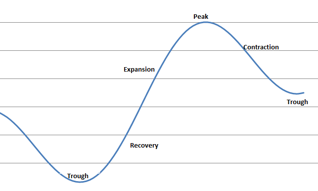
There are five main phases of the economic cycle that are commonly recognized:
1. Expansion: This phase is characterized by economic growth, rising employment, increased production, consumer spending, and business investments. It typically includes increasing GDP, low inflation, and stable interest rates.
2. Peak: The economy reaches its maximum level of development and growth, with further growth potentially leading to overheating. In this phase, prices of goods and services reach their highest levels, and the growth of profits and employment begins to slow down.
3. Recession/Contraction: The economy begins to decline after reaching its peak. During a recession, there is a reduction in production, worsening employment figures, and a decrease in demand for goods and services, which can lead to a decline in company profits and a rise in unemployment levels.
4. Trough: In this phase, the economy reaches its lowest point and begins to rise. Demand for goods and services starts to recover, and the growth of profits and employment gradually improves.
5. Recovery: The economy begins to recover after reaching the trough. Production, company profits, and employment figures improve, leading to renewed growth and expansion.
Discussions typically focus on the growth and recession of the economy, classifying phases where the economy is either expanding or contracting. To better understand this, let's examine the stock market's performance during periods of recession and around the beginning and end of these phases.
The standard approach is to use the timing of recessions as determined by the National Bureau of Economic Research (NBER). In total, 15 recessions have been identified since 1927. The logarithmic graph below displays market returns with recessions depicted as gray areas to highlight these periods.
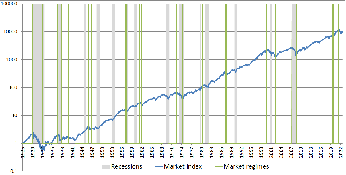
The Compound Annual Growth Rate (CAGR) of the US stock market over the entire period was 10%, with a Sharpe ratio of 0.53. The total return reached nearly one million percent (more precisely, 990,000%, excluding dividend reinvestment).
If the economy was in a recession, the market was also bearish in 55% of the cases. Conversely, when there was no recession, the market was bearish in only 13% of the cases. Since 1926, the total time spent in recessions has been approximately 17%.
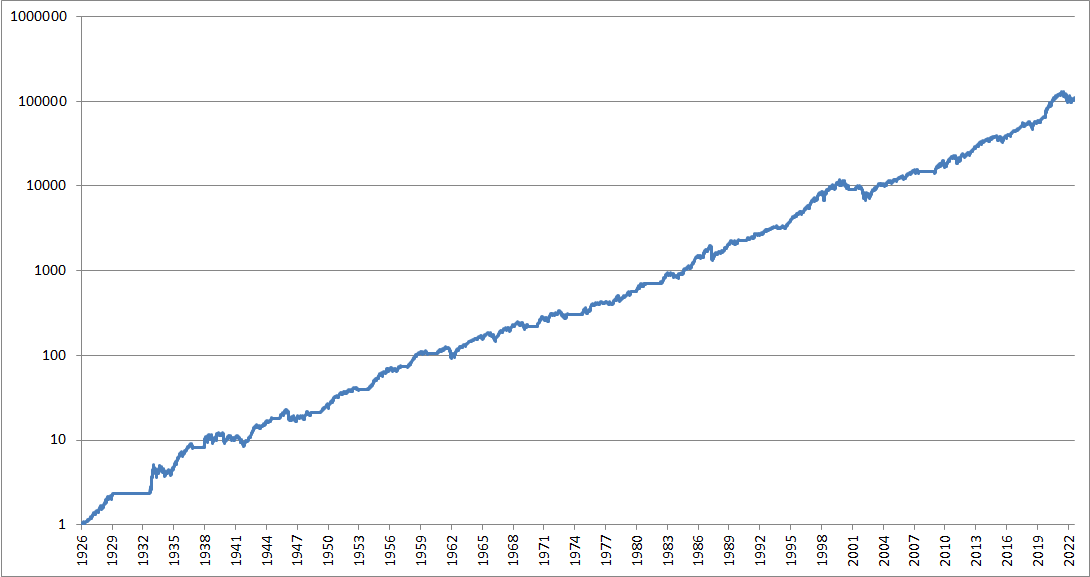
Exiting the market at the beginning of a recession and re-entering it at its end would have increased the CAGR to 12.7% and the Sharpe ratio to 0.86, as shown in the diagram below:
Furthermore, exiting investments prior to a recession can provide even greater improvements. The table below demonstrates various scenarios for timing market exits before a recession (t) with a certain lag in months.
Exiting the market relative to the beginning of a recession, with re-entry into the market at the end of it:
| Full period | Begin - 6m | Begin - 3m | Begin - 1m | Begin + 0m End - 0m | Begin + 1m | Begin + 3m | Begin + 6m | |
| CAGR | 10% | 12.5% | 12.6% | 12.9% | 12.7% | 12.4% | 11.5% | 11.1% |
| Sharpe | 0.53 | 0.88 | 0.86 | 0.88 | 0.86 | 0.83 | 0.73 | 0.69 |
To further analyze the returns, it's important to consider different re-entry points into the market relative to the end of recessions. In this case, we always exit positions at the beginning of a recession and re-enter at end + t.
Re-entering the market relative to the end of a recession, with an exit at the beginning of it:
| End - 6m | End - 3m | End - 1m | Begin + 0m End + 0m | End + 1m | End + 3m | End + 6m | |
| CAGR | 13.3% | 13.8% | 13.1% | 12.7% | 11.8% | 10% | 9.1% |
| Sharpe | 0.8 | 0.87 | 0.83 | 0.86 | 0.81 | 0.73 | 0.68 |
As it can be seen from the tables above, the ability to identify, or even better, predict, recessions has historically had a positive effect on portfolio returns. The scenario that comes closest to an optimal entry/exit strategy is to exit the market one month before the beginning of a recession and re-enter three months before it ends. This scenario yields a CAGR of 14% and a Sharpe ratio of 0.89. However, even exiting the market at the beginning of a recession already leads to a significant improvement in performance. In this case, the annualized return increases from 10% to 12.7%, which amounts to an impressive 9.7 million percent over the period from 1926, compared to the market's actual return of roughly one million percent.
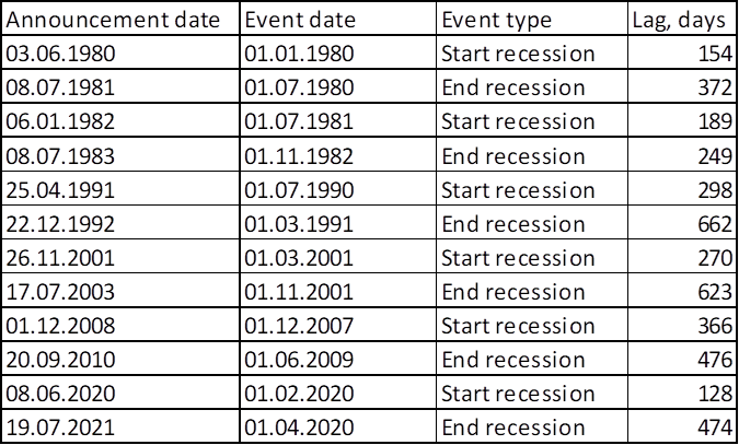
While it may seem that there is a relatively simple solution to beat the market — exit when the NBER announces the beginning of a recession and re-enter when it announces its end — it's not that straightforward. The NBER's announcements regarding economy peaks and troughs are significantly delayed. The NBER's Business Cycle Dating Committee is responsible for determining the beginning and end dates of recessions. The committee typically waits several months after the start of a recession to declare that one has occurred, as it needs time to analyze and confirm the data.
The NBER defines a recession as "a significant decline in economic activity spread across the economy, lasting more than a few months, normally visible in real GDP, real income, employment, industrial production, and wholesale-retail sales." In other words, a recession is a period of economic contraction characterized by a decrease in economic output, employment, and other key indicators of economic activity. This means that relying solely on the NBER's announcements may not provide a timely and efficient strategy for adjusting one's investment positions.
The lag in NBER announcements for the last six recessions is shown in the table below:
Since relying on NBER announcements about the beginning of a recession is impractical due to their delayed nature, the question arises about constructing a coincident or, even better, a leading indicator to determine the phases of the economic cycle.
One of our goals in macro analysis is to search for methods that enable us to predict or timely identify the state of recession in real time. A potential solution could be the use of Dynamic Factor Models (DFM), which identify a common hidden factor in a set of indicators.
DFM is a time-series model that allows for the aggregation of several macro indicators into a single, comprehensive economic indicator, which can be used to determine the current stage of the cycle. Importantly, this approach helps to deal with the problem of high dimensionality in macro data, which occurs when the number of available indicators exceeds the number of periods for which historical data is available.
In our approach to determining the economic state, we employ DFM that incorporates the following economic factors:
- Industrial production
- Retail sales
- Unemployment
- Consumer Price Index
- Broad stock market yield
During the testing process, we use vintage data for all macro indicators to avoid look-ahead bias. In the current scenario, the application of DFM provides a comparable quality of recession forecasting, with an accuracy of 94%. The chart below displays the fluctuations of our DFM indicator in relation to recessions, which are highlighted in gray. We can clearly see that when the indicator goes into negative territory, the probability of recession increases.
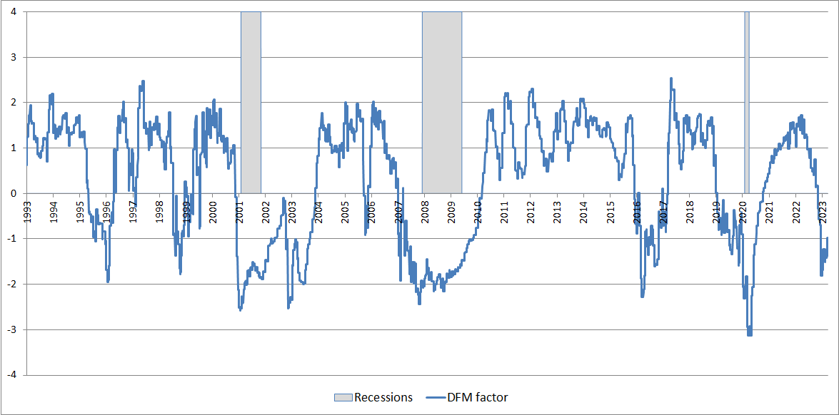
However, the economy was in recession only 17% of the time, and using the zero line as a threshold would result in numerous false predictions. Therefore, we shift the threshold further into the negative zone to improve accuracy.
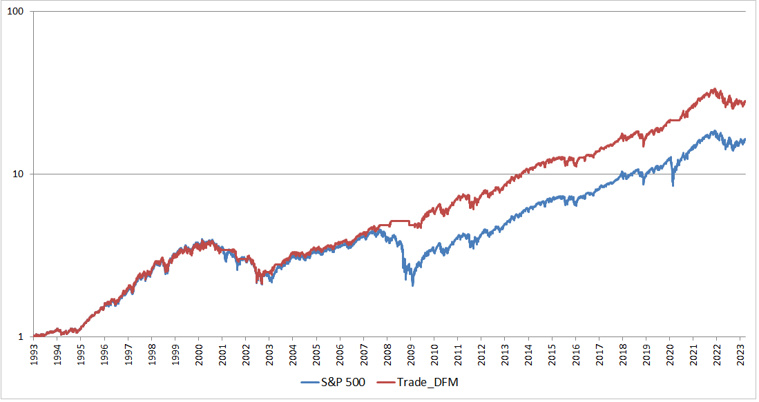
Remaining out of the market whenever our DFM indicator falls below the threshold for the period 1993-2023 would yield the following results in comparison to the S&P 500 index:
| CAGR | Sharpe ratio | |
| S&P 500 | 9.70% | 0.49 |
| Trade_DFM | 11.64% | 0.72 |
From the table above, we can see that the DFM indicator adds value by increasing both the Annualized return and the Sharpe ratio. The diagram below demonstrates that the DFM indicator was successful in filtering out some pronounced market downturns while taking advantage of the overall market uptrend.
Macro-based timing methods, like the one presented in this article, can enhance investment outcomes compared to a base index. However, they should not be the only component of a comprehensive trading strategy. A well-rounded approach should also incorporate mechanisms for selecting optimal investment instruments and implementing hedging techniques.